SWOT

The Surface Water and Ocean Topography (SWOT) mission will launch in 2021, and will measure surface water (especially rivers and lakes), globally. All rivers greater than 100 m wide will be measured, with the potential to get down to rivers as small as 50 m in width. SWOT will produce measurements of river height, slope, and width. Our group has been focusing on rivers.

In comparison with in situ gages, measuring rivers with a radar allows you to see all big rivers in the world, but with different space, time, and noise characteristics. When averaged over 1 km² of river area, river height precision will be 10 cm. SWOT’s orbit will repeat every 21 days; in each 21 day cycle, an average point in the mid-latitudes will be measured twice. At higher latitudes, there will be far more measurements. Measurements will be irregular in time. However, entire long profiles of water elevation will be imaged with a single snapshot. 

In order to help future users to better understand SWOT data, our group has produced an example data product over six months of the Sacramento River. This example data product was constructed from a detailed hydraulic simulation, and run through similar processing steps as will be used in the SWOT mission. However, this has not been produced by the exact software used by the SWOT project at JPL, so it is not an “official” example data product. We only are sharing and describing the “vector” data products, that is the data after they have been mapped onto a 1-D river channel. The below shows the three passes that sample the Sacramento River, as well as our study domain:

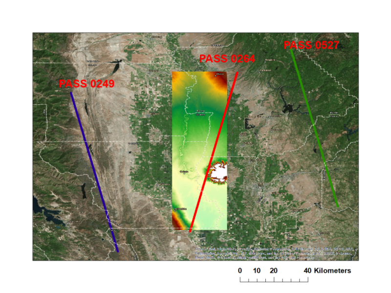
Of these three, Pass 264 passes directly over the study area, and thus much of the river is not observed, as the SWOT measurements will be made in a swath between 10-60 km on either side of the nadir ground track. SWOT measurements will not be acquired in the so-called “nadir gap”. Passes 249 and 527 both observe the river fairly well, although some of the most westerly portions of the river fall just outside the far swath for pass 527. The example data product includes all three. 

The example data product construction begins with a 1-D shallow water simulation of six months on the Sacramento River using the HEC-RAS model. River XS are available for this river, and the model has been calibrated by the USGS. We then mapped the water elevations from 1-D into 2-D using the RAS Mapper, combined with a 3 m LiDAR DEM. For each SWOT overpass time, we pushed 2-D maps of water and land elevations into the SWOT instrument simulator, which simulates low-level radar interaction with the land media. Note: the data we are sharing here includes residual errors due to uncorrected wet tropospheric delay, and errors due to so-called cross-over calibration. This data also include errors due to layover, and thermal noise. It does not include so-called “dark water”, nor to riparian vegetation.

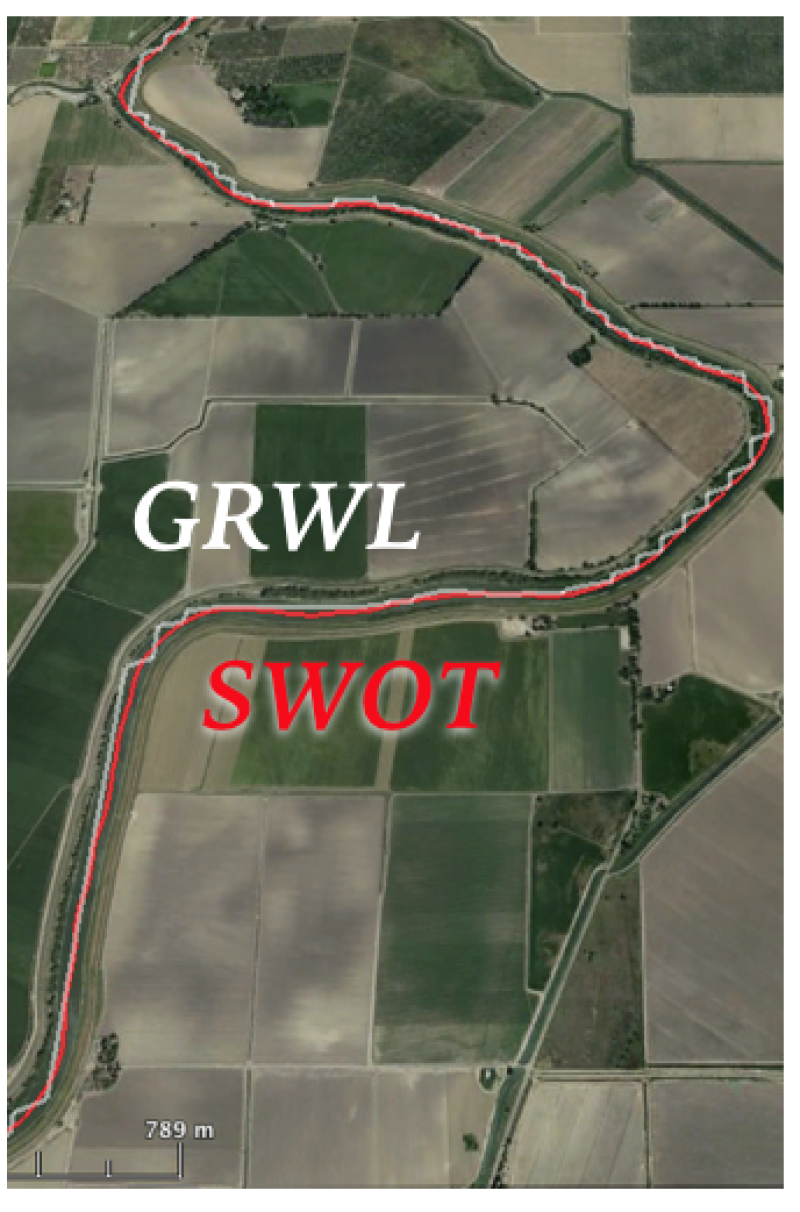
Once the SWOT simulator produces a map of radar pixels, SWOT hydrology processing begins. Pixels are averaged and geolocated, and then mapped onto river centerlines. The river centerlines themselves are built starting from the Global River Widths from Landsat (GRWL) dataset from Tamlin Pavelsky and George Allen (UNC and JPL, respectively). GRWL centerlines are refined based on pixels from several SWOT overpasses. The figure below shows the GRWL and SWOT centerlines.

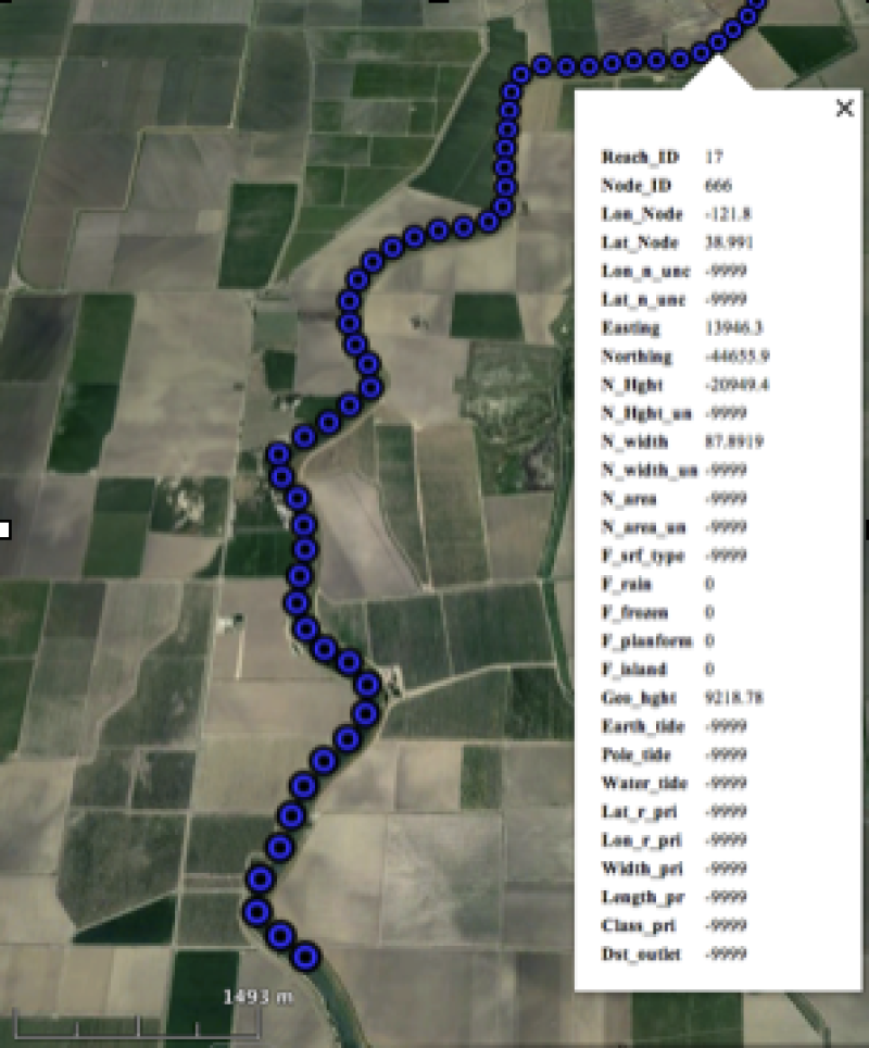
Once pixels are associated with centerlines, they are assigned to particular “nodes”, which are located at 200 m intervals along the centerline. This is done using the open source RiverObs software (link) originally by Ernesto Rodriguez, JPL.

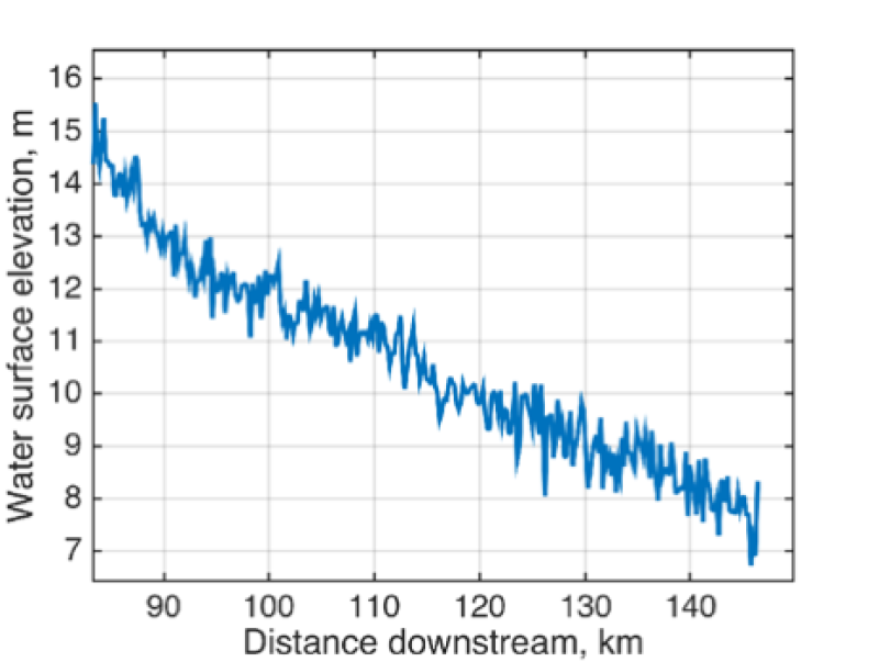
Node data are relatively noisy (~35 cm RMSE for height, and ~18 m error for width, with significant variability across the swath). The below image shows node-level heights for the downstream portion of the simulated domain.

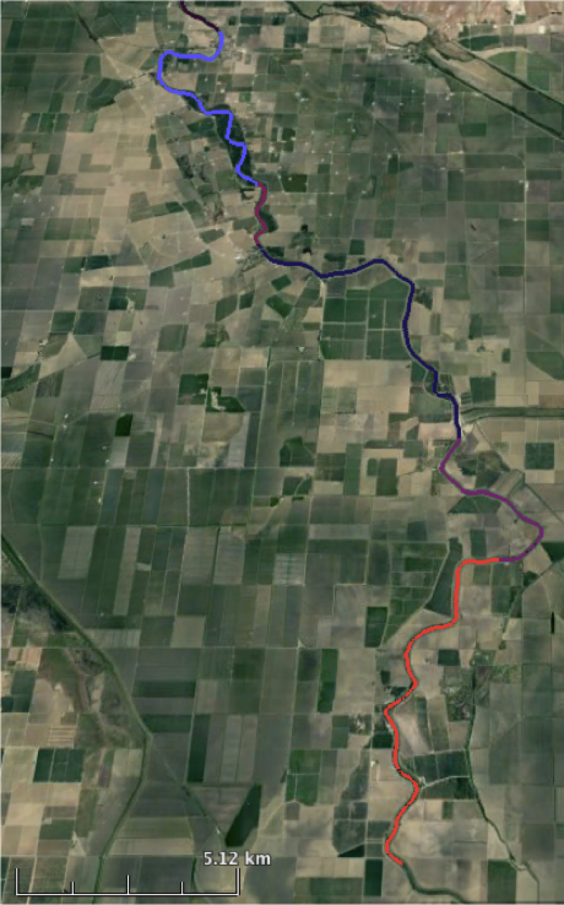
Finally, node data are gathered into reaches, which are ~10 km in length, and represent an averaging area over which SWOT measurements are relatively precise. Below are several reaches shown by color, in the downstream part of the domain.

Notes on production: 

• We used a height error model to predict uncertainty: node uncertainty = 40 cm if < 60 km, and = 100 cm if > 60 km. This is a placeholder for now; we are currently working to improve this with JPL.
• Partial domain observations: if SWOT doesn’t see any pixels for a given node, or any nodes for a given reach, they aren’t in the truth or the data product at all. Additionally, if a node doesn’t meet certain criteria (>100 pixels available to compute height, e.g.), then the data element (e.g. node height) is listed as -9998. Plan to adapt this in the future to combine with the error model.
• Many data elements are not yet produced by RiverObs: these are listed as -9999 for the time being.

You can obtain the processed dataset here (link). Unzipping will produce a directory with datafiles. They were produced using Rui’s slightly modified branch of RiverObs (link), with a few tweaks and fixes not currently incorporated into the main RiverObs branch.

Notes on the dataset: 

• Slides presented at the June 2018 SWOT Science Team meeting, revised October 2018 (Day1P_1630_RiverObs_Rev.pdf). 
• Brief description of each field (data element) (Metadata.xlsx). This describes filenames, as well as data elements, and error codes.
• The data product is presented in shapefile (.shp) format. 
• There are separate files for the “Truth”, which is the data products but without any SWOT noise added. This allows users to explore the level of noise for nodes and reaches.
• The “rdf” directory includes the configuration files for RiverObs so that users can reproduce these results.

We have also provided a way to quickly pull all data into Matlab and compute errors as compared with the truth dataset; it generates most of the figures produced in the Science Team slides mentioned above. You can grab this from Rui’s GitHub here. A direct link to a pdf view of all of the comparisons produced is here.

Enjoy. We would greatly appreciate it if you would let us know you are looking at the dataset, by emailing Mike at durand.8@osu.edu.